Final post

I ended up generating something not bad…

Of course it faded away but still 🙂

Again, the learning curve and the spectrogram:

The step in the train curve is due to a change of training subset (I don’t compute the cost on the whole training data) when I restarted the learning.

The seed ended at one second and we can see that it generates something «good» for two seconds (from 1 to 3) before getting stuck in a fixed point. Its interesting since I propagated the gradient for two seconds during the training.

The last day

Using lasagne I was able to produce something more interesting with a small (200 to 100 to 100 to 200) LSTM.  Thanks to Christopher Beckham’s blog and repo for helping me understand the RNN part of lasagne in about 2h. Everything that I do in lasagne can be found in the «Last try» folder in my repo.

Its just one long note but its the best that I generated so far. Let’s take a look at the learning curves and the spectrogram:

Here is the seed and the generated sequence. We can see that the model get the highest frequency and produce it. The problem is that it got stuck in a fix point and produces the same thing over and over.

I have now an idea on why my previous models didn’t work. I think it has to do with the way I generate my batches. I used to take my batches from the data set completely at random and now (following what Christopher did) to generate a batch I take one element at random and I complete the batch by shifting it. I think it’s important since by doing this the model can learn more easily to be equivariant to shifts (if it receive a shifted input it will produce a shifted output) and that is a property we want.

I’m training a larger model right now and at the time I don’t think it will reach a small enough mean square error. My last post will probably be on this model.

Last week

I’m still not able to produce a long sequence of sound…

You can see here what is the best sound I generate so far

I had no time to test in the frequency domain, I spend all my time training a lot of different models in the time domain and nothing worked out… I tried the following too see where is the problem:

• Check if the non-linearities were saturated
• Check if the way I generated the batches was fine
• Check if my implementation of RMSprop was doing the same thing as other implementations
• Check and double-check if everything is well linked in my implementations of LSTM and GRU

And everything seems fine.

I tried a lot of things:

• Used GRU and LSTM
• Varying the number of layers from 1 up to 5
• Varying the number of hidden units from 200 up to 2000
• Varying inputs length from 200 up to 32000
• Varying the sequence length from 6 up to 60
• etc…

which end up producing three different things:

1. Nothing (no sound)
2. Noise (like the end of what is shown here but louder)
3. One note and then noise… (which is the best I got)

As presented in a previous post, the strategy was always the same; train the model to predict what’s next and then, using a seed, use the predictor as a generator.

Here is the spectrogram of the seed concatenated to what I generated. You can easily guess where the generation started…

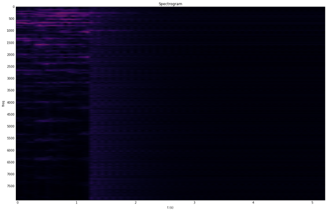
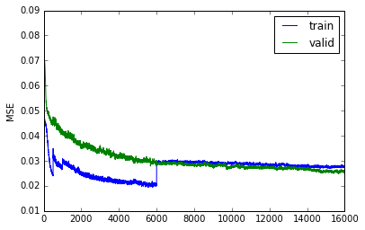
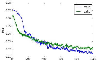
Even though it’s really bad and unimpressive it still menages to get some frequency right before fading away. The model which does it is a three layers GRU with no end layer (the top hidden cell is directly use in the cost). Maybe the model is just not train enough as shown by the learning curve (on the valid set) here:

which seems to still go down, just really, really slowly. It took one whole day to train this model on a GPU.

I really don’t know where it goes wrong and if I had to restart it over I’ll definitely use a library like lasagne or blocks. It was probably not a great idea the rebuild the wheel to solve directly this task but I will for sure make it work this summer by first testing my code on a standard data set like TIMIT. I should have realize earlier that I wouldn’t have the time to make it work and start using a library but I didn’t.

Tomorrow I will try lasagne and hopefully produce something.

week: 28 march (part 2)

Though on the frequency domain

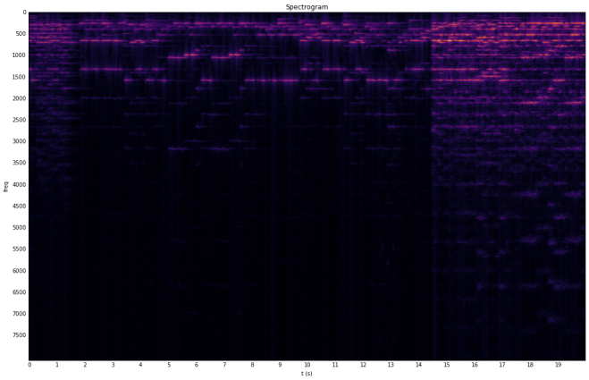
In the frequency domain we have two numbers by frequency. Often these two numbers are represented as a complex number. However, when plotted in the obvious way (i.e. we plot Re(c) and Im(c)), it’s hard to see any pattern. In my opinion, the best representation of these two numbers  is the amplitude and the phase. The amplitude gives us the information about which note is played: We can see the pattern in the amplitude of the frequency of this Mozart piece. The problem is the phase… I don’t believe that there’s a model that can reproduce such a thing. But do we need to reproduce exactly that? No, not exactly. For instance if we reproduce this up to a global phase it will not be noticeable. The only thing that is important is the relative phases.

Another question that is important to ask about the phase reconstruction is what kind of metric do we use? d(x, y) = (x-y)² is probably not our best choice… d(π, –π) = (π – –π)² = 4π² ≈ 39.47 while π and –π are the same in radian… we would like to have a metric that has those properties:

• d(θ, φ) = d(θ+2nπ, φ+2mπ) for all integer n, m
• d(θ, φ) = d(θ+w, φ+w) for all w
• d(0, π) ≥ d(θ, φ) for all θ, φ
• d(θ, φ) = 0 iff there is n an integer s.t. θ+2nπ = φ
• and the usual metric properties (without d(θ, φ) = 0 iff θ = φ)

d(θ, φ) = sin²((θ – φ)/2) has those properties. I think it’s worth a try.

So what’s next?

1. Try the first strategy (as presented bellow) on the amplitude of the frequency domain to see if these model is enough.
2. If it’s not enough try a more powerful model such as D.R.A.W.
3. See if phase reconstruction is possible using the amplitude

 

week: 28 march

Explaining what I did so far:

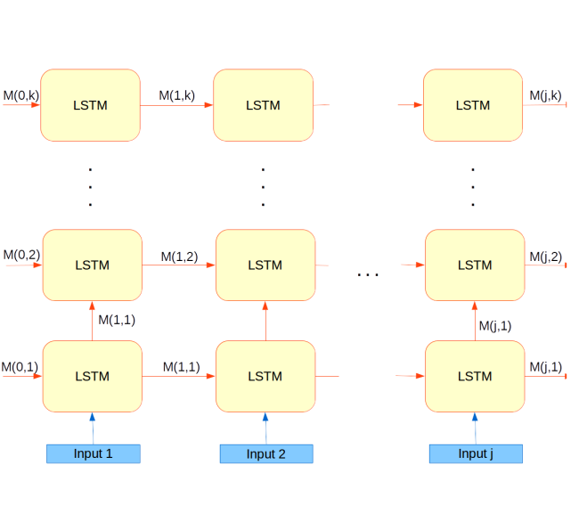
Everything has been done in the time domain and I used LSTM in all experiments. The input size and the value of k are hyperparameters. When I train those model I usually backpropagated through 2 seconds i.e. I calculated the gradient on 32 unfolds if the input size is set to 1000 for example.

For the cost function I used two strategies:

1.  Concatenated for all k M(i, k) to predict the next input i.e. Input i using a one hidden layer MLP (which was train with the LSTM)
2. Concatenated for all k M(i, k) to reconstruct the current input (still with a MLP) with a noisy LSTM

I wasn’t able to train the LSTM with the first strategy to produce something interesting (it produces noise). The second strategy on the other hand was able to produce the right frequency and overtones (as we can see in the last post) but it fails at being creative since it only finds a fixed points and always reproduces the same thing (it was train to reproduce its input after all).

I also found out that bigger models doesn’t mean better results, or perhaps I’m just bad at training larger models. Every model I train got stuck at the same minimum.

Week: 21 march

I used a variant of the LSTM with noise injection and depth 2 to generate the next 0.015625 second at every steps.

Here is the original spectrogram  vs a sampled one.

This slideshow requires JavaScript.

It was clearly under train, the training curve was still going down (it still got some notes and their overtones). But now I’m more confident that it works and I can train a bigger model!

Week: 1 february

Updating MLP and gradient descent and adding a sound test which uses Fourier transform.

Week 3

Homework 1 is done and pushed on GitHub, I achieve 98% accuracy on test set using rectifier, normalization and a PCA.

Week 2

I programmed a simple MLP and used it for classification on MNIST. I used cross-entropy and stochastic gradient descent with early stopping. I got 97.7% accuracy on the test set and it took less than 5 minutes on ipython with a 4 years old standard laptop to train.

Everything is on GitHub.

GitHub

https://github.com/duchesneaumathieu/IFT6266.git